
Market dispersion refers to the variation in returns of the market’s underlying securities. Opportunities for successful security selection abounds when market dispersion is high, as discussed before. Here we explain the methodology for calculating an asset-weighted standard deviation of share returns, often also referred to as the cross-sectional standard deviation.
This measure describes the dispersion in individual stock returns. If we want to examine how market dispersion affects manager outperformance we have to measure the dispersion of active portfolio returns instead. I will discuss this in a following post. However, as preparation, we first consider market dispersion from a stock perspective.
As before, performance is measured against the unbiased market-capitalisation (market-cap) weighted benchmark. The analysis is also applicable when we compare managers against their peers.
We consider a simplified stock market which consists of two large-capitalisations (cap) and two small-cap stocks. Stock A and Stock B have market caps equal to 45% and 35% respectively of the market’s total capitalisation. Stock C and D have market caps of 10% and 5% respectively of the total market. The stock weights and benchmarks returns for a measurement period are given in the graphs below:

The market cap-weighted benchmark return is calculated as
Benchmark return 
where 


To assist with our explanation we now graph the stocks’ performances, relative to the benchmark, on the x-axis versus their market-caps on the y-axis.

The simplest measure of security dispersion is to calculate the range of returns between, top performing and bottom performing groups of securities, such as quartiles. In our case, the difference between the best and worst performing shares is, for example, 20%.
Here I rather use a more comprehensive measure that incorporates the degree of variation of all stock returns relative to the benchmark. Hence we calculate the differences, as shown in the graph, between each security’s return and the benchmark return:
i’th security’s return – market-cap benchmark’s return 
with 
Next, we aggregate these differences, but to ensure that the positive and negative values do not cancel out, we either have to use the absolute values of the differences or the squares of the differences. Either approach can be used. I prefer to use the squared differences because the results are more accentuated. They are also more useful for calculating multi-period dispersion, a topic I will consider in a future post.
Our aim is to measure the amount by which the outperformance of a randomly selected stock deviates from the benchmark, on average. When summing the squared differences we, therefore, have to weigh each share’s out- or underperformance by its market cap. This is because the share’s market-cap gives the probability that it will be picked at random. The graph above can, therefore, be interpreted as a probability distribution function as found in statistics.
To better understand the reasoning behind the weighing process let’s divide our illustrative market into 20 equally weighted components, each with a market cap of 5%. Stock A is subdivided into 9 components, Stock B into 7 components and Stock C into 2 components. So, along with stock D, the market then consists of 20 equally weighted components. The market’s dispersion can now be calculated as the sum of the 20 components’ deviations from the benchmark. This is identical to calculating a weighted sum of their deviations from the benchmark.
The squared differences, loaded by market cap, is called the asset-weighted variance or cross-sectional variance. To ensure that market dispersion is measured in the same units as the security returns we take the square root of the sum. Then, market dispersion, represented by the symbol 
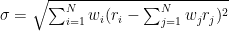
with N the total number of securities. This is called the asset-weighted standard deviation or cross-sectional standard deviation (see, for example, here). In our example the asset weighted dispersion is

This is a measure of the amount by which a randomly selected stock’s out- or underperformance deviates from the benchmark, on average. As discussed in the next post we are actually interested in how randomly selected portfolio’s out- or underperformance deviates from the benchmark.